
Whether you've been using Excel for years, or just a few months, here are our 5 Excel tips that everyone should know.
Want to watch bite-sized videos instead? Watch free Excel tutorials on Learnreel now!
1. Transforming data into an interactive database
Table formatting may seem like a simple tool, but it is one that few people take advantage of. Table formatting allows you to take your data range and turn it into an interactive database, making it easier to analyse data.
【Table Formatting in Excel】
To set up a table, click on any cell in your dataset, and then select [Home] > [Format as Table].
Choose your colour scheme and then make sure the relevant data is selected and you have the box ticked if your data includes headers.
With your database ready, you can easily sort and filter data.
【Table Formatting in Google Sheet】
Select your data range, and then click [Format] > [Alternating Colors].
Choose your colour scheme and have the box ticked if your data includes headers.
For sorting and filtering data, click on arrow in specific column for further actions (eg. sort data from A-Z)
2. Simplifying complex data for reports with Paste Special
Without using complicated formulas, you can automatically simplify data in a worksheet using the Paste Special command.
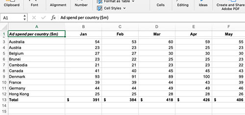
【Summarise the data from full numbers to millions of dollars in Excel】
Rather than dividing each cell manually by 1,000,000, use Paste Special!
Follow these 4 steps:
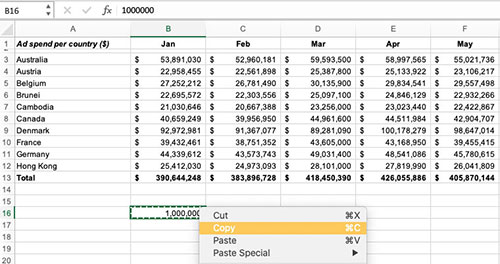
1】First type the amount you want to divide the data by and then right click and copy the cell.
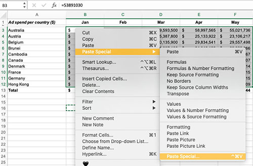
2】Next, select the data range you want to simplify, being careful not to select the bottom row which sums the data. Right click, press Paste Special and choose paste special again.
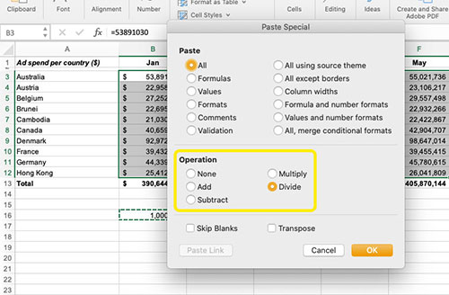
3】In Operation, select the function you want to use. Here you want to divide all data by the one million you copied earlier.
4】Once your data has been simplified, you can change the width of the columns and delete the cell you copied. Remember to also change the units on the table.
(Note:Paste Special is currently not available in Google Sheet. Please refer to the next function!)
3. Locking a cell when copying formulas with absolute references
The “$” dollar sign in a cell reference affects just one thing - it instructs Excel how to treat the cell when the formula is moved or copied to other cells.
【Absolute references in Excel & Google Sheet】
Here we have data that we want to convert to another currency. Using a simple formula, we multiply the original currency by the exchange rate.
However, when we try to copy that formula to the rest of our dataset, Excel automatically updates all parts of the formula.
We can use the $ sign before the row and column coordinates to lock the cell reference.
▶ [B3*$B$12]
Then, when we copy the formula, the locked cell reference does not change.
You can use this function in any situation where you need to multiply or divide numbers by one specific cell, as well as many other uses.
4. Turning copied data into columns (Text to Columns)
If you copy a block of data from a webpage, a word processing file, or other text file, all the data is dumped into a single column of cells.
To make this data usable, you need the text to columns function.
【Text to Columns in Excel】
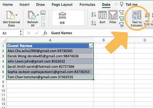
1】Select your data range and then go to [Data] > [Text to Columns]
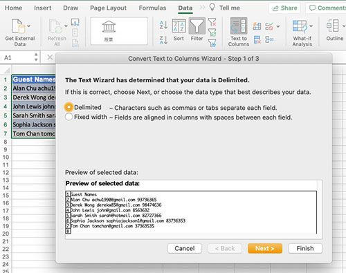
2】If your data is divided by spaces or commas, choose “Delimited”
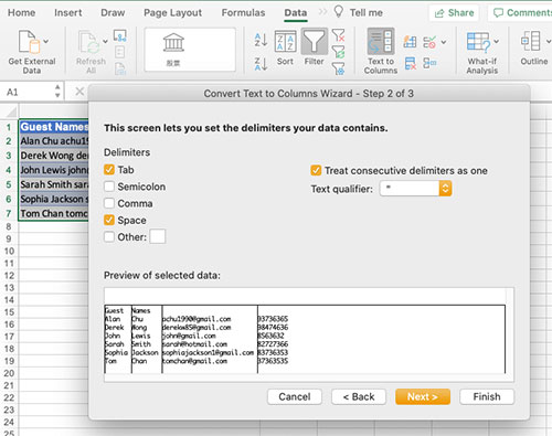
3】Excel will automatically choose how to divide your data. If this looks correct then click next and check the formatting of the data is also correct before clicking finish
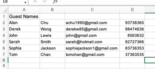
4】Your data is now in columns, ready for further work.
【Text to Columns in Google Sheet】
[Data] > [Split text to columns]
Choose the specific [Separator] on how to divide your data. For example, you could choose Space / Detect automatically.
5. Combining data using &
Combining cells is easy when they’re numbers, you simply add the cells together.
However, when you have text to combine, you need to use the ‘&’ function between the cells you want to combine.
【Combining text cells in Excel / Google Sheet】
For text, if you also want a space between the combined cells, then insert a space between two quotation marks, followed by another & symbol.
▶ [A2&“ ”&B2]
You can use this function to add any number of cells together and quotation marks to add spaces or set text between the combined cells.
Discover short courses, videos and tips & tricks on Learnreel for $0.
Learnreel is a TikTok-style app where you can learn from experts through short, actionable videos. Find out more here.